Table of Contents
- What Is a Microscope Camera and How It Integrates with Your Optics?
- Key Image Quality Factors: Resolution, Sampling, and Pixel Size
- Sensor Technologies Compared: CCD, CMOS, and sCMOS Trade-offs
- Color, Monochrome, and Spectral Fidelity for Light Microscopy
- Dynamic Range, Noise, and Sensitivity in Low-Light Imaging
- Frame Rates, Rolling vs Global Shutter, and Motion Artifacts
- Optical Coupling and Adapters: C-mounts, Relay Lenses, and FOV Matching
- Choosing by Application: Brightfield, Fluorescence, Stereo, and Metallurgy
- Connectivity, Software, and File Formats: Practical Workflow Considerations
- Budgeting and Total Cost of Ownership: Where to Spend
- Frequently Asked Questions
- Final Thoughts on Choosing the Right Microscope Camera
What Is a Microscope Camera and How It Integrates with Your Optics?
A microscope camera is a digital imaging device designed to capture the intermediate image formed by your microscope’s optical system. Unlike a general-purpose camera, a microscope camera is optimized for stable mounting on a phototube or eyepiece tube, precise parfocality with visual observation, and a data interface and software stack suitable for measurement, analysis, and documentation. Choosing the right camera is ultimately an exercise in optical matching (sensor size and pixel size to objective and adapter), signal management (noise, dynamic range, sensitivity), and workflow (frame rates, software, formats).

Effie Alberta Read, Ph. D, M. D., Assistant Chief of the Microanalytical Laboratory, prepares a microphotographic camera. She was an authority on microscopic methods in the examination of food and drugs who joined the agency in 1907 and remained until her death in 1930. For more information on FDA History, please visit: www.fda.gov/AboutFDA/WhatWeDo/History/default.htm
To choose well, it helps to understand the imaging path:
- Objectives form a magnified, diffraction-limited image of the specimen.
- In infinity-corrected systems, a tube lens converts collimated light into an intermediate image; in finite systems, the objective directly forms the intermediate image at a defined tube length.
- A camera relay (often a C-mount adapter such as 0.5× or 1.0×) further scales this intermediate image onto the camera sensor.
- The sensor samples the optical image into pixels, constrained by sampling theory and noise.
Every decision—sensor size, pixel pitch, adapter magnification, and bit depth—affects what you actually see in the saved image. A camera that is superb for dim fluorescence may be overkill (and overly expensive) for brightfield teaching; a camera that produces smooth video for live demonstrations may not capture enough detail for quantitative measurements. The sections below unpack each factor and connect them to realistic use cases.
Key idea: The best microscope camera is the one that correctly samples the optical resolution you already own and moves data to your computer at the speed and fidelity your work demands.
As you read, look for cross-references to topics like optical coupling and field of view and dynamic range and noise. These are the practical levers that make the difference between a camera that just works and one that works brilliantly in your setup.
Key Image Quality Factors: Resolution, Sampling, and Pixel Size
Resolution in a microscope image is limited by the optics, not the camera. The objective’s numerical aperture (NA) and the wavelength of light (λ) determine the finest resolvable detail in widefield (incoherent) imaging. A commonly used lateral resolution criterion is approximately:
- Rayleigh criterion (lateral): ~ 0.61 × λ / NA
While the optical system creates resolution, the camera must sample that detail without losing information. Nyquist’s sampling theorem states that to represent the highest spatial frequency passed by the optics, the camera’s sampling interval at the specimen plane should be small enough:
- For incoherent imaging, the optical cutoff frequency is approximately fc ≈ 2 NA / λ (cycles per unit length).
- Nyquist requires sampling at least twice this frequency, so the effective pixel size at the specimen should satisfy Δx ≤ 1 / (2 fc) ≈ λ / (4 NA).
The effective pixel size at the specimen is simply the camera pixel pitch divided by the total magnification between specimen and sensor (objective × any relay/adapter magnification and tube-lens scaling in infinity systems):
# Given

pixel_size_um      # camera pixel pitch in micrometers (µm)

objective_mag      # e.g., 10x, 20x, 40x ...

adapter_mag        # e.g., 1.0x, 0.63x, 0.5x (relay lens)

# For infinity systems with non-standard tube lens, include the ratio:

# total_mag = objective_mag * adapter_mag * (tube_lens_f / reference_f)
# Effective sampling at the specimen plane

effective_pixel_um = pixel_size_um / total_mag
# Nyquist guideline for incoherent imaging

nyquist_step_um = wavelength_um / (4 * NA)

# Aim for: effective_pixel_um <= nyquist_step_um

Equivalent circuit of the CMOS Image Sensor pixel
Color sensors with a Bayer filter mosaic sample each color channel more sparsely than a monochrome sensor, because each pixel measures only one color and color information is reconstructed algorithmically. To preserve fine detail across channels, it is often beneficial to slightly oversample (smaller effective pixel size) compared with a monochrome camera used at the same wavelength.
Megapixels vs. meaningful detail
Megapixel counts can be misleading in microscopy. If your optics and sampling are limiting resolution to a certain value at the specimen plane, increasing the sensor’s pixel count without adjusting pixel size or magnification just creates larger files—not more real detail. Two practical points help frame expectations:
- Optical resolving power sets the ceiling. No camera can recover detail the optics never delivered.
- Field of view (FOV) scales with sensor size. When sampling is already adequate, a larger sensor increases the area you capture in one frame without altering the smallest resolvable feature size.
If your primary goal is to capture a larger region at the same optical resolution, choose a larger sensor and the appropriate adapter magnification to avoid vignetting and preserve sharpness to the corners. If your goal is to capture finer detail, revisit NA, wavelength, and pixel size together rather than chasing megapixels alone.
Sensor Technologies Compared: CCD, CMOS, and sCMOS Trade-offs
Digital microscope cameras today predominantly use CMOS and scientific CMOS (sCMOS) sensors. CCD sensors historically dominated certain scientific markets, but modern sCMOS has displaced many CCD use cases thanks to favorable noise, speed, and size characteristics. Here’s what matters for selection, without veering into brand- or model-specific claims:

One of the first active pixel sensors (aka. CMOS sensor)
CCD (Charge-Coupled Device)
- Strengths: Mature technology; historically valued for uniformity and low fixed-pattern noise in some applications.
- Limitations: Generally slower readout compared with modern sCMOS; higher power; fewer current options; often smaller formats today.
CMOS (Complementary Metal-Oxide Semiconductor)
- Strengths: High frame rates; on-sensor processing flexibility; broad range of sensor sizes and pixel pitches; cost-effective.
- Limitations: Rolling shutter is common; fixed-pattern noise characteristics vary with design and processing.
sCMOS (Scientific CMOS)
- Strengths: Low read noise, high quantum efficiency (particularly in back-illuminated designs), high frame rates, large sensors with many pixels.
- Limitations: Price; large data volumes; some models still use rolling shutters (though global shutters are available in certain sensors).
In practical terms, if you need fast acquisition, low noise, and large FOV, sCMOS is often the default choice. For budget-conscious teaching, documentation, and routine brightfield, standard CMOS-based cameras are widely used and perfectly capable when matched to optics and sampling requirements discussed in Resolution, Sampling, and Pixel Size.
Keep in mind that terms like “quantum efficiency,” “read noise,” and “dark current” describe intrinsic sensor behavior that impacts low-light performance and dynamic range. For demanding fluorescence imaging, these sensor-level attributes matter as much as pixel size and optics. For brightfield documents and classrooms, the illumination is typically abundant, and other factors (color fidelity, ease of use, and software) often rank higher.
Color, Monochrome, and Spectral Fidelity for Light Microscopy
One of the earliest choices is whether you need a color or monochrome camera. The right answer depends on your specimens, illumination, and analysis goals.
Color cameras (Bayer or similar color filter arrays)
- Use when: Recording naturalistic images (brightfield of stained tissues, educational materials, materials with visible colors), sharing live demonstrations, or publishing color figures.
- Considerations: Demosaicing reconstructs full-color pixels from a mosaic; spatial resolution for individual color channels is effectively reduced compared with a monochrome sensor of the same pixel pitch. Slight oversampling (see Sampling) can help restore apparent detail.
- White balance and color profiles: Accurate white balance, illumination stability, and color management in software are crucial for faithful reproduction.
Monochrome cameras
- Use when: Imaging fluorescence, phase contrast for quantitative analysis, polarized light where intensity is the primary readout, or any application where signal-to-noise and resolution are paramount.
- Considerations: No color filter array means all pixels collect light across the sensor’s sensitivity band, improving sensitivity and avoiding color reconstruction artifacts. If you later need color, you can add filters and acquire sequential channels, but that is a different workflow than one-shot color.
Spectral considerations
- Illumination spectrum: Ensure your light source is suitable for the wavelengths of interest. For example, fluorescence channels require excitation and emission filters tuned to fluorophore spectra; brightfield benefits from a stable, broad-spectrum source.
- Sensor spectral response: Sensors differ in sensitivity across wavelengths. If you work heavily in a specific band (e.g., near-UV or near-IR), review the sensor’s relative response in that region and ensure compatible optics.
For mixed workflows—say, occasional fluorescence plus routine brightfield—some users maintain both a monochrome and a color camera on swappable ports. If you only want one camera, decide which mode is the priority. Color cameras can certainly record bright fluorescence, but monochrome is typically preferred for quantitation and sensitivity in low-light channels.
Dynamic Range, Noise, and Sensitivity in Low-Light Imaging
Dynamic range and noise determine how faithfully your camera records weak and strong signals in the same scene. In microscopy, this matters for both brightfield (preserving highlights in bright backgrounds while maintaining contrast in faint features) and fluorescence (detecting dim emitters without saturating brighter structures).
Key definitions
- Full-well capacity (FWC): The number of photoelectrons a pixel can store before saturating. Larger pixels generally hold more charge, supporting greater dynamic range if noise is low.
- Read noise: Electronic noise added during readout. Lower read noise helps in low-signal regimes.
- Dark current: Thermally generated electrons accumulating during exposure. Cooling can reduce dark current and stabilize the baseline in long exposures.
- Dynamic range: Often expressed as the ratio FWC/read noise (sometimes converted to decibels). Higher is better for scenes with mixed brightness.
- Bit depth: The number of discrete digital levels (e.g., 12-bit, 14-bit, 16-bit). Higher bit depth supports finer intensity gradations, but it does not by itself increase the sensor’s analog dynamic range—it encodes it.

Unknown CMOS image sensor, probably OmniVision, in a glass chip-scale package. The top cover glass is visible, the active imaging area is the dark rectangle framed by a gold line. CMOS logic is hidden beneath a light-blocking layer with a purple appearance in this image. Package size is about 4x4.5 mm with 5x6 balls (presumably 30 contacts). Resolution is 640x480, active area 2.3x2.9 mm, which suggests 1/5\" OF.
In well-lit brightfield with short exposures, read noise and dark current are less critical; illumination typically dominates the signal. In low-light scenarios (e.g., weak fluorescence), read noise and quantum efficiency are crucial. The interplay among pixel size (larger pixels collect more photons at a given irradiance), exposure time, and illumination intensity determines whether your signal rises sufficiently above noise.
Practical tips for selecting by noise and dynamic range
- If you often see highlight clipping or loss of shadow detail in brightfield, consider a camera with higher dynamic range and ensure you are using adequate sampling while avoiding overexposure.
- For dim fluorescence, low read noise and high sensitivity dominate selection. Cooling becomes useful when exposures are long enough for dark current to matter.
- Choose bit depth appropriate to your analysis. For quantitative work, higher bit depths help capture subtle intensity differences; for routine documentation, 8–12 bit pipelines may suffice, depending on software.
Remember: Bit depth encodes what the sensor can deliver. If the analog signal is noisy or clipped, more bits won’t restore lost information.
Frame Rates, Rolling vs Global Shutter, and Motion Artifacts
Frame rate requirements vary widely. Live classroom demonstrations benefit from smooth real-time video at modest resolutions. High-speed phenomena or scanning workflows demand higher frame rates and low latency. Three interrelated factors shape your camera’s temporal performance:
- Sensor readout architecture: Determines maximum frames per second (fps) at given resolutions and bit depths.
- Shutter type: Rolling shutters expose and read rows sequentially; global shutters expose the full frame simultaneously.
- Data interface: USB 3.x, Gigabit Ethernet (GigE), 10GigE, and other interfaces limit sustained throughput and may affect latency; see Connectivity.
Rolling vs global shutter
- Rolling shutter: Most common in CMOS and sCMOS cameras; fine for static or slowly changing scenes. Can produce skew or partial-exposure artifacts if the subject moves or the illumination is modulated during readout.
- Global shutter: Exposes all pixels simultaneously; preferred when motion-induced distortion must be minimized (e.g., rapidly moving micro-organisms or mechanically scanned stages).
If you occasionally capture motion but mostly record static specimens, a rolling-shutter sCMOS may be entirely sufficient and offers advantages in noise and cost. If your workflow frequently involves motion or pulsed light synchronized to exposure, evaluate global-shutter options and triggering features.
Optical Coupling and Adapters: C-mounts, Relay Lenses, and FOV Matching
Getting the image from the microscope to your sensor requires attention to mechanics and optics. Most microscope cameras attach via a C-mount thread. Between the phototube and the camera, a relay lens (adapter) scales the intermediate image so your sensor sees a suitable field of view (FOV) without vignetting, while maintaining parfocality with the eyepieces.
Adapter magnification and sensor size
- Common adapter magnifications: 1.0× (no additional relay magnification), 0.7×, 0.63×, 0.5× and others.
- Goal: Match the sensor’s diagonal to the microscope’s image circle available at the camera port. Too small an adapter (e.g., 0.35× on a large sensor) risks vignetting; too large (e.g., 1.0× on a small sensor) limits your captured FOV unnecessarily.

Pentax 12mm f/1.2 C-Mount TV lens with a C-Mount to CS-Mount adapter
Microscope phototubes are often optimized for sensor formats around 1/2″ to 2/3″. Larger sensors can still be used but may require specific phototubes and adapters designed for a wider image circle to avoid corner shading and aberrations. Always verify that your chosen adapter is specified for your microscope’s optical system (finite vs infinity, tube lens focal length) so that intermediate image geometry remains correct.
Eyepiece projection vs dedicated camera port
- Eyepiece projection: Adapters that slip into the eyepiece tube are convenient for occasional imaging or microscopes lacking a camera port. They can be more sensitive to alignment, and FOV may be more restricted.
- Phototube/camera port: Provides a stable, parfocal, and typically wider field, especially on research-grade stands. Preferred for permanent setups and measurement workflows.
Field number, FOV, and sampling
While eyepieces are specified by a field number (FN, in millimeters), camera FOV is determined by the sensor size and the relay optics. If you want your camera image to match as closely as possible to what you see through the eyepieces, choose the adapter to project a comparable image circle onto the sensor. Then ensure your effective pixel size meets the sampling criteria for your objectives and wavelengths.
Finally, check back focal distance and parfocality adjustments on your adapter. Achieving parfocality (camera and eyepieces in focus simultaneously) improves ergonomics and speeds up imaging sessions.
Choosing by Application: Brightfield, Fluorescence, Stereo, and Metallurgy
Once you’re comfortable with sensor concepts and optical coupling, filter them through real-world use. The optimal microscope camera for one application may be suboptimal for another. Here are practical guidelines for common modalities:
Brightfield and phase contrast (well-lit, visible light)
- Priorities: Accurate color (if needed), good dynamic range to preserve highlights, comfortable frame rate for live focusing.
- Pixel size: Choose to meet or slightly exceed the Nyquist sampling guideline for your highest-NA objective you plan to image with.
- Sensor size: Larger sensors capture more FOV—useful for scanning and documentation.
Fluorescence (low-light, narrowband emission)
- Priorities: High sensitivity, low read noise, stable dark signal; monochrome sensors are typically preferred.
- Cooling: Consider cooling when exposure times are long enough for dark current to accumulate.
- Bit depth: Higher bit depth supports quantitative work; pair with low-noise sensors to realize the benefit.
Stereo and macro microscopy (large working distance, 3D specimens)
- Priorities: Wide FOV, comfortable live video, color fidelity if inspecting colored parts.
- Optical coupling: Stereo phototubes and dedicated adapters vary widely; match adapter magnification to sensor size to capture the available field without vignetting.
- Depth of field: Remember depth of field constraints; camera choice doesn’t change DOF physics, but higher frame rates help when z-stacking via focus stacks.
Reflected-light materials/metal microscopy
- Priorities: High contrast, dynamic range to handle specular highlights, accurate color (if relevant), and low noise for differential interference contrast (DIC) imaging.
- Polarization: If using polarized light, a monochrome camera can be advantageous for intensity analysis; color is fine for documentation.
For time-lapse or scanning stages, revisit frame rate and shutter needs and consider software automation features covered in Connectivity and Software. The best selection aligns the sensor’s strengths with your highest-impact imaging mode while remaining serviceable for secondary tasks.
Connectivity, Software, and File Formats: Practical Workflow Considerations
The best sensor in the world is of limited use if data arrives too slowly or software impedes your work. Evaluate the full data path from the sensor to your storage and analysis tools.
Interfaces and bandwidth
- USB 3.x: Common, plug-and-play, adequate for many cameras. Ensure your computer port and cable match the camera’s specified speed class and power needs.
- GigE/10GigE: Longer cable runs and network integration; good for distributed setups. Bandwidth depends on link speed; 10GigE supports higher data rates than standard GigE.
- Direct-to-monitor HDMI: Useful for presentations; typically independent of raw data capture to a computer. Check if simultaneous HDMI view and USB capture are supported in your system.
Drivers and software features
- Acquisition control: Exposure, gain, white balance (for color), gamma/transfer functions, ROI selection, and binning.
- Image processing: Flat-field correction, shading correction, denoising, and color calibration. These should be optional and transparent so raw data remains available for quantitative work when needed.
- Measurement tools: Calibration management, scale bars, annotations, and reporting workflows.
- Automation hooks: SDKs or scripting interfaces for time-lapse, z-stacks, tiling, and hardware triggers. For motion-sensitive work, verify trigger input/output options and timing characteristics.
File formats and data management
- Raw vs processed: Prefer saving in a lossless, metadata-rich format when you need to retain quantitative integrity; use compressed formats for documentation and sharing.
- Bit depth and color space: Ensure exported files preserve the camera’s bit depth when required. For color, manage white balance and profiles consistently to avoid mismatches between screens and prints.
- Storage and throughput: High-resolution, high-frame-rate imaging generates large datasets. Plan for SSD speed, disk capacity, and backup strategies.
Where possible, test software with your own workflow: focus, capture, annotate, measure, export. Small usability wins (like responsive live view and intuitive ROI selection) save time in every session.
Budgeting and Total Cost of Ownership: Where to Spend
Microscope camera pricing spans a wide range. Spend where it will make a sustained difference in your images and your time. Consider both initial cost and total cost of ownership (TCO), including adapters, software, and support.
Prioritize optical match and sensor fundamentals
- Get sampling right first: Choose pixel size and adapter magnification that meet the Nyquist sampling guideline for your most-used objective(s) and wavelengths.
- Buy sensitivity only if you need it: Low-noise, high-sensitivity sensors are invaluable for dim fluorescence; for brightfield teaching or inspection, you can redirect budget to sensor size (FOV), software features, or ergonomics.
- Plan for data: If you adopt large, fast sensors, budget for storage and compute to keep pace.
Hidden and adjacent costs
- Adapters and phototubes: A well-matched relay lens can transform image quality and FOV. Confirm compatibility with your microscope’s optical system.
- Calibration and maintenance: Periodically verify scale calibration and parfocality. Keep relay lenses clean; dust and smudges degrade contrast.
- Support and updates: Software longevity and OS compatibility matter over the lifetime of the camera.

Microscope with LM digital adapter (www.micro-tech-lab.com) and Canon EOS 350D mounted to a phototube (C-mount thread), and Olympus E330 / E-510 attached to an ocular tube
When comparing options across budgets, make a short list of non-negotiables (e.g., monochrome sCMOS if you do fluorescence) and a list of nice-to-haves (e.g., global shutter, larger sensor for additional FOV). This helps prevent overspending on features that yield little benefit in your actual work.
Frequently Asked Questions
How many megapixels do I need for a microscope camera?
There is no universal “right” megapixel count. What matters most is whether your effective pixel size at the specimen meets the Nyquist sampling guideline for your optical resolution (set by NA and wavelength). Once sampling is sufficient, more pixels primarily increase the field of view captured by enlarging the sensor, not the smallest resolvable detail. If your goals are documentation and larger FOV, a higher-megapixel, larger sensor is beneficial. If your goals are finer detail, consider higher-NA objectives or shorter wavelengths in addition to pixel considerations.
Should I choose a 0.5× or 1.0× C-mount adapter?
It depends on your sensor size and the microscope’s available image circle. A 0.5× adapter projects a larger portion of the intermediate image onto the sensor, increasing FOV for a given sensor size—useful with small to medium sensors, provided you don’t introduce vignetting. A 1.0× adapter maintains the microscope’s native projection and can suit larger sensors or phototubes designed for wide fields. The practical choice is to match the sensor diagonal to the phototube’s image circle and verify that your effective pixel size still satisfies sampling requirements at your target objectives.
Final Thoughts on Choosing the Right Microscope Camera
Buying a microscope camera is less about chasing specs and more about matching physics to purpose. Start with your optics (NA, objectives, wavelengths), determine the sampling you need at the specimen plane, and then select a sensor and adapter that deliver that sampling across a suitable field of view. From there, balance noise, dynamic range, and frame rate against your actual workflow—brightfield documentation, live demonstrations, or low-light fluorescence imaging.
If you remember one formula, let it be the Nyquist guideline for incoherent imaging: effective pixel size at the specimen should be on the order of λ/(4×NA) or smaller. Pair that with the practical advice in Optical Coupling and Adapters and the workflow checks in Connectivity and Software, and you’ll be well-equipped to choose confidently.
Want more evidence-based guides like this? Explore related topics in our fundamentals and accessories series, and subscribe to our newsletter to get future deep-dives, practical checklists, and application notes delivered to your inbox.